Visualization of bird sound files on amplitudes
import matplotlib.pyplot as plt
import numpy as np
import pandas as pd
import os
from pydub import AudioSegment
from scipy import signal
from scipy.io import wavfile
# custom matplotlib style
usetex = True
fontsize = 14
params = {'axes.labelsize': fontsize + 2,
      'font.size': fontsize + 2,
      'legend.fontsize': fontsize + 2,
      'xtick.labelsize': fontsize,
      'ytick.labelsize': fontsize}
      #'text.usetex': usetex} # Requires latex on the computer
plt.style.use('ggplot')
plt.rcParams.update(params)
Pre-processing
Conversion: MP3 to WAV
Here, we take all the MP3 bird sounds inside the "ALL BIRDS" and "Test Birds from Kasios" folders, and convert them into WAV files.
We have to do this because WAV is the most supported format to do sound processing.
Please put the folders "ALL BIRDS" and "Test Birds from Kasios" of the VAST challenge in the folder "data".
from data.loader import get_kasios_obs, get_obs, map_path

df = get_obs(songs = True)
df_kasios = get_kasios_obs(songs = True)
Visualization
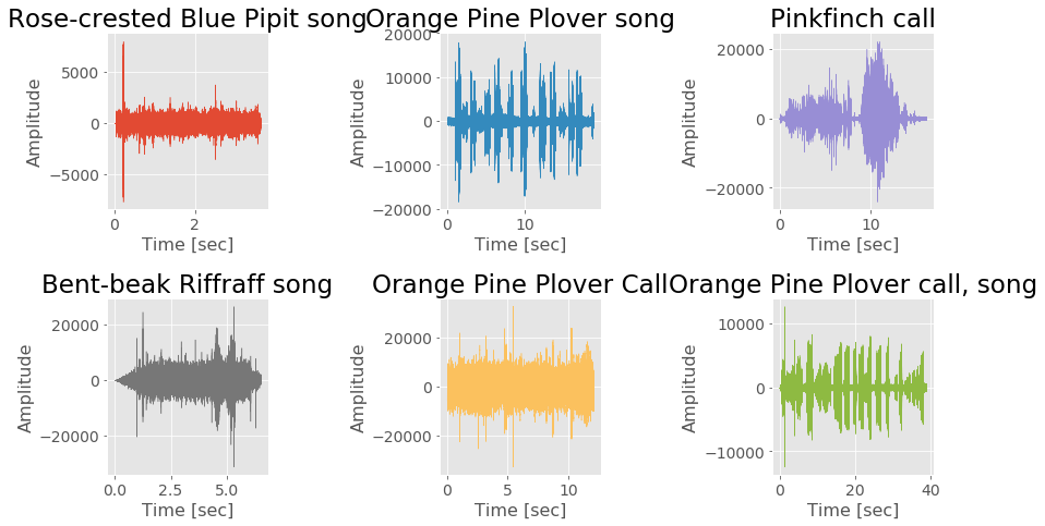
Temporal representation
# take random samples
samples = df.sample(6)

fig = plt.figure(figsize=(13,7))
for i, (index, obs) in enumerate(samples.iterrows()):
    # read wav file
    rate, data = wavfile.read(obs["song"])

    times = np.arange(len(data))/float(rate)
    title = '{} {}'.format(obs["English_name"], obs["Vocalization_type"])

    ax = fig.add_subplot(2, 3, i+1)
    ax.fill_between(times, data, color="C{}".format(i)) # plot the signal
    ax.set_title(title)
    ax.set_xlabel('Time [sec]')
    ax.set_ylabel('Amplitude')

plt.tight_layout()
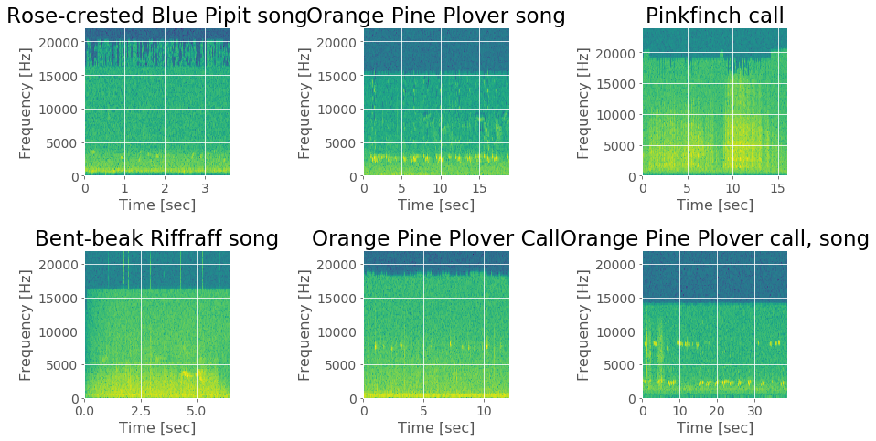
Frequency representation (2D spectrogram)
fig = plt.figure(figsize=(13,7))
for i, (index, obs) in enumerate(samples.iterrows()):
    # read wav file
    rate, data = wavfile.read(obs["song"])

    times = np.arange(len(data))/float(rate)
    title = '{} {}'.format(obs["English_name"], obs["Vocalization_type"])

    ax = fig.add_subplot(2, 3, i+1)
    ax.specgram(data, Fs=rate)
    ax.set_title(title)
    ax.set_xlabel('Time [sec]')
    ax.set_ylabel('Frequency [Hz]')

plt.tight_layout()
Analyze Kasios test birds with visualizations
Kasios provided 15 birds sounds. According to them, they are songs and calls from the Rose-crested Blue Pipit species.
Aim: Analyse the Kasios birds tests records and verify from which species each record belongs.
The dataset we have been provided contains 186 samples of Rose-crested Blue Pipits sounds. They are "songs" and "calls", with different qualities, graded from A to E. Most of them are in good quality. In fact, quality A and B represent 148 records.
We will first visualize some of the Blue Pipits records to identify some characteristics, and then we will compare what we obtained with the Kasios records.
To do the comparison, we will plot all the records with the same scales. The time (x-axis) will go from 0 to 20 seconds, and the amplitude (y-axis) from -10000 to 10000.
def plot_signal_temp(df, title):
    fig = plt.figure(figsize=(13,9))
    fig.suptitle(title)
    for i, (index, obs) in enumerate(df.iterrows()):
        # read wav file
        rate, data = wavfile.read(obs["song"])

        times = np.arange(len(data))/float(rate)
        title = '{} {}'.format(obs["English_name"], obs["Vocalization_type"])

        # plot the signal
        ax = fig.add_subplot(3, 3, i+1)
        times = np.arange(len(data))/float(rate)
        ax.fill_between(times, data, color="C{}".format(i))
        ax.set_xlabel('Time [sec]')
        ax.set_ylabel('Amplitude')
        ax.set_xlim(0, 20)
        ax.set_ylim(-10000, 10000)

    fig.tight_layout(rect=[0, 0.03, 1, 0.95])

def plot_spectrogram(df, title):
    fig = plt.figure(figsize=(13,9))
    fig.suptitle(title)
    for i, (index, obs) in enumerate(df.iterrows()):
        # read wav file
        rate, data = wavfile.read(obs["song"])

        times = np.arange(len(data))/float(rate)
        title = '{} {}'.format(obs["English_name"], obs["Vocalization_type"])

        # plot the spectrogram
        ax = fig.add_subplot(3, 3, i+1)
        ax.specgram(data, Fs=rate)
        ax.set_xlabel('Time [sec]')
        ax.set_ylabel('Frequency [Hz]')
        ax.set_xlim(0, 20)

    fig.tight_layout(rect=[0, 0.03, 1, 0.95])
Blue Pipit songs
df_bp_songs = df.loc[(df['English_name'] == 'Rose-crested Blue Pipit')
                     & (df['Vocalization_type'] == 'song')
                     & (df['Quality'] == 'A')]
df_bp_songs = df_bp_songs[:9]


display(df_bp_songs)

plot_signal_temp(df_bp_songs,
                 title='Rose-creasted Blue Pipit songs')
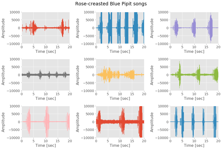
In the different records, the time of silence varies, but the time of the songs is approximately the same (2 seconds).
The amplitude of the song periods is going crescendo.
Blue Pipit calls
df_bp_calls = df.loc[(df['English_name'] == 'Rose-crested Blue Pipit')
                    & (df['Vocalization_type'] == 'call')
                    & (df['Quality'] == 'A')]
df_bp_calls = df_bp_calls[:9]


display(df_bp_calls)

plot_signal_temp(df_bp_calls,
                 title='Rose-creasted Blue Pipit calls')
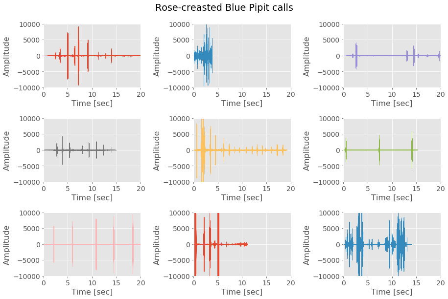
We can distinguish the repetition of high amplitude picks followed by silences.
These picks events are the calls. They happen at regular intervals.
Kasios files
# Get all tests sounds of Kasios
fig = plt.figure(figsize=(17,15))
fig.suptitle('Kasios test files')

for i, (index, obs) in enumerate(df_kasios.iterrows()):
    # read wav file
    rate, data = wavfile.read(obs["song"])

    # plot the signal
    ax = fig.add_subplot(5, 3, i+1)
    times = np.arange(len(data))/float(rate)
    ax.fill_between(times, data, color="C{}".format(i%9))
    ax.set_xlabel('Time [sec]')
    ax.set_ylabel('Amplitude')
    ax.set_xlim(0, 20)
    ax.set_ylim(-10000, 10000)

fig.tight_layout(rect=[0, 0.03, 1, 0.95])
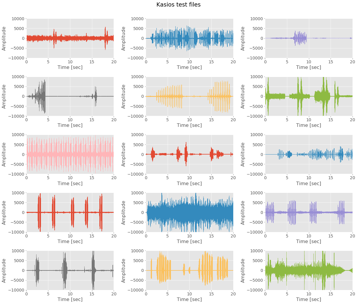
From the shapes of Blue Pipit songs and calls we have just described, we can say that most of the test files do not look like Blue Pipit records.
On the next plot, we emphasize this in focusing on each test sound one by one. We will try to say if it looks similar to a Blue Pipit call or song.
fig = plt.figure(figsize=(15,40))
fig.suptitle('Test file : Is a Blue Pipit record or not ?')

f = df.loc[368492].song
rate_calls, data_calls = wavfile.read(f)
f = df.loc[377874].song
rate_songs, data_songs = wavfile.read(f)


for i, (index, obs) in enumerate(df_kasios.iterrows()):
    # read wav file
    rate, data = wavfile.read(obs["song"])

    # visualize the signals
    ax = fig.add_subplot(15, 3, 3*i+1)
    times = np.arange(len(data))/float(rate)
    title = 'Kasios test {}'.format(i+1)
    ax.fill_between(times, data, color="C{}".format(i%9))
    ax.set_title(title)
    ax.set_xlim(0, 20)
    ax.set_ylim(-10000, 10000)

    bx = fig.add_subplot(15, 3, 3*i+2)
    times = np.arange(len(data_calls))/float(rate_calls)
    bx.fill_between(times, data_calls, color="C{}".format(i%9))
    bx.set_title('Blue Pipit call')
    bx.set_xlim(0, 20)
    bx.set_ylim(-10000, 10000)

    cx = fig.add_subplot(15, 3, 3*i+3)
    times = np.arange(len(data_songs))/float(rate_songs)
    cx.fill_between(times, data_songs, color="C{}".format(i%9))
    cx.set_title('Blue Pipit song')
    cx.set_xlim(0, 20)
    cx.set_ylim(-10000, 10000)

fig.tight_layout(rect=[0, 0.03, 1, 0.95])
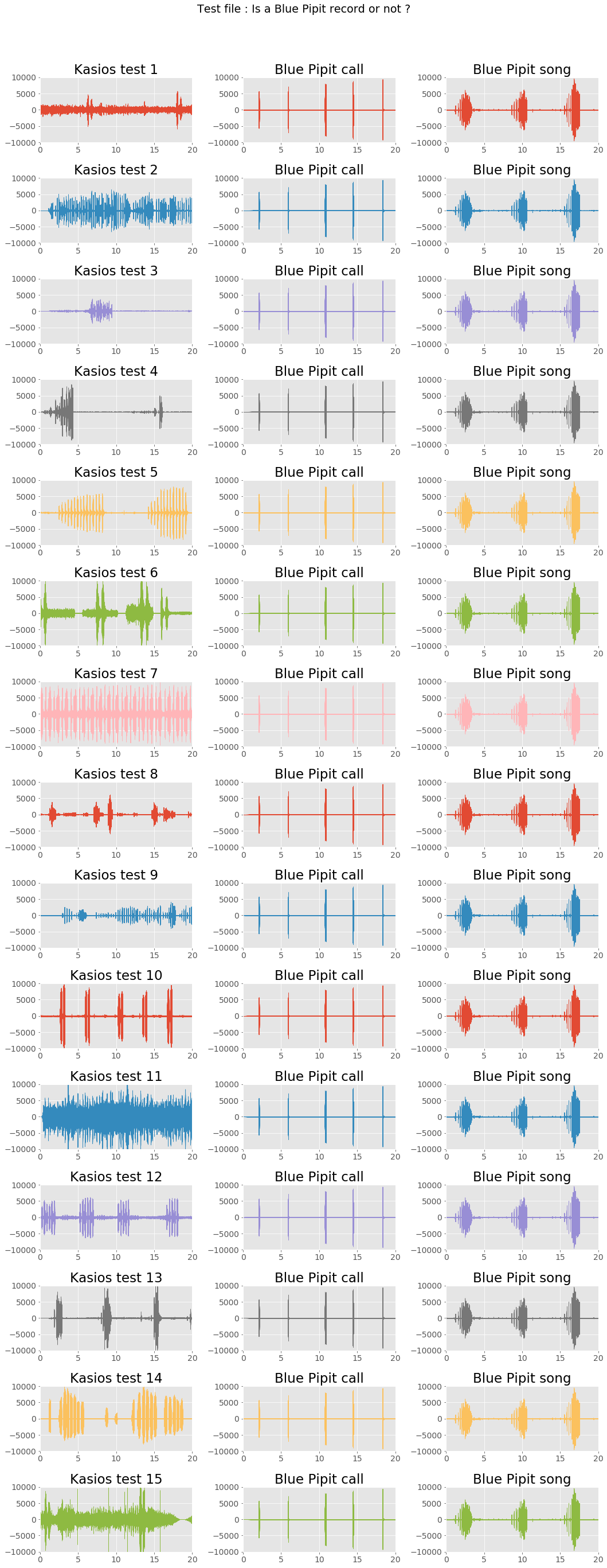
| Test file | Looks similar to Blue Pipit |
|---|---|
| 1 | Yes |
| 2 | No |
| 3 | No |
| 4 | Maybe |
| 5 | No |
| 6 | No |
| 7 | No |
| 8 | No |
| 9 | No |
| 10 | No |
| 11 | Maybe |
| 12 | No |
| 13 | Yes |
| 14 | No |
| 15 | Yes |
Check the notebook 4_spectral_analysis.ipynb.