Classification of the sound with Machine Learning and visualization
Import and load data
In [1]:
from lib.File import File
from matplotlib import pyplot as plt
from data.loader import get_kasios_obs, get_obs, map_path
import numpy as np

from math import sqrt
import pandas as pd
In [2]:
# Loads files and makes conversion if necessary
df_all = get_obs(songs = True)
df_kasios = get_kasios_obs(songs = True)
In [3]:
# X = get_spectres(df_all) # Can be very long
# X.to_pickle("data/all_birds_freq.pickle") # Save to cache
X = pd.read_pickle("data/all_birds_freq.pickle") # Quicker to use cache

X.head()
Out[3]:
In [4]:
# X_kasios = get_spectres(df_kasios) # Can be very long
# X_kasios.to_pickle("data/kasios_birds_freq.pickle")
X_kasios = pd.read_pickle("data/kasios_birds_freq.pickle") # Quicker to use cache

X_kasios.head()
Out[4]:
In [5]:
Y = df_all.English_name
Y_bin = df_all.English_name == "Rose-crested Blue Pipit"
In [6]:
from sklearn.model_selection import train_test_split, cross_val_score
from sklearn.metrics import accuracy_score,recall_score,confusion_matrix

X_train, X_test, y_train, y_test = train_test_split(X, Y, test_size = 0.33)
X_bin_train, X_bin_test, y_bin_train, y_bin_test = train_test_split(X, Y_bin, test_size = 0.33)
In [7]:
from sklearn.neighbors import KNeighborsClassifier
In [8]:
#creating odd list of K for KNN
#myList = list(range(1,50))
# subsetting just the odd ones
#neighbors = filter(lambda x: x % 2 != 0, myList)
neighbors = list(range(1,50,2))
# empty list that will hold cv scores
cv_scores = []
# perform 10-fold cross validation
for k in neighbors:
knn = KNeighborsClassifier(n_neighbors=k)
scores = cross_val_score(knn, X_bin_train, y_bin_train, cv=10, scoring='accuracy')
cv_scores.append(scores.mean())
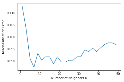
# changing to misclassification error
MSE = [1 - x for x in cv_scores]
# determining best k
optimal_k = neighbors[MSE.index(min(MSE))]
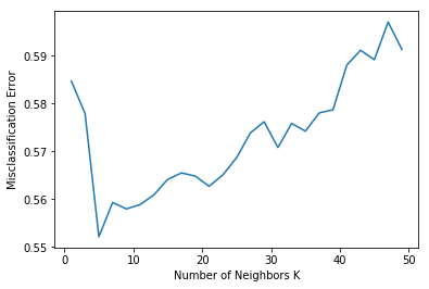
print("The optimal number of neighbors is %d" % optimal_k)
# plot misclassification error vs k
plt.plot(neighbors, MSE)
plt.xlabel('Number of Neighbors K')
plt.ylabel('Misclassification Error')
plt.show()
In [9]:
clf = KNeighborsClassifier(n_neighbors=optimal_k)
clf.fit(X_bin_train, y_bin_train)
Out[9]:
In [10]:
# Accuracy of the model
accuracy = clf.score(X_bin_test, y_bin_test)
print("Accuracy of the model: %s" % accuracy)
In [11]:
import itertools
import numpy as np
import matplotlib.pyplot as plt

from sklearn.model_selection import train_test_split
from sklearn.metrics import confusion_matrix


def plot_confusion_matrix(cm, classes,
                          normalize=False,
                          title='Confusion matrix',
                          cmap=plt.cm.Blues):
    """
    This function prints and plots the confusion matrix.
    Normalization can be applied by setting `normalize=True`.
    """
    if normalize:
        cm = cm.astype('float') / cm.sum(axis=1)[:, np.newaxis]

    plt.imshow(cm, interpolation='nearest', cmap=cmap)
    plt.title(title)
    plt.colorbar()
    tick_marks = np.arange(len(classes))
    plt.xticks(tick_marks, classes, rotation=45)
    plt.yticks(tick_marks, classes)

    fmt = '.2f' if normalize else 'd'
    thresh = cm.max() / 2.
    for i, j in itertools.product(range(cm.shape[0]), range(cm.shape[1])):
        plt.text(j, i, format(cm[i, j], fmt),
                 horizontalalignment="center",
                 color="white" if cm[i, j] > thresh else "black")

    plt.ylabel('True label')
    plt.xlabel('Predicted label')
    plt.tight_layout()
In [12]:
# Compute confusion matrix
y_bin_predict = clf.predict(X_bin_test)
cnf_matrix = confusion_matrix(y_bin_test, y_bin_predict)
np.set_printoptions(precision=2)
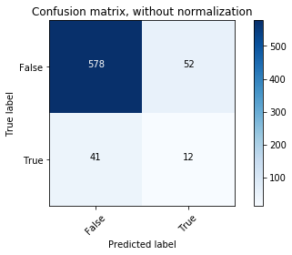
# Plot non-normalized confusion matrix
plt.figure()
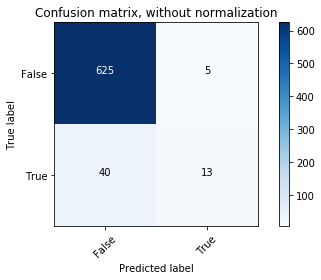
plot_confusion_matrix(cnf_matrix, classes=[False,True],
title='Confusion matrix, without normalization')
# Plot normalized confusion matrix
plt.figure()
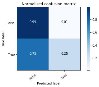
plot_confusion_matrix(cnf_matrix, classes=[False,True], normalize=True,
title='Normalized confusion matrix')
plt.show()

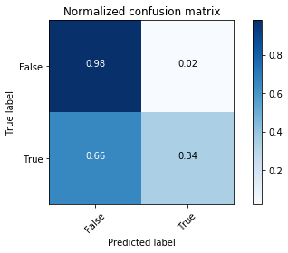
The classifier is not able to recognize most of the Rose-crested Blue Pipit species. It may be overfitting.
Predicting
In [13]:
print("Binary classification with kNN \n")
y_kasios = clf.predict(X_kasios)
for i in range(len(y_kasios)):
    print("Kasios song n°%s : %s" % (i+1, y_kasios[i]))
The kNN classifier has detected the Kasios song n°9 as a Blue Pipit one.
In [14]:
from sklearn import svm
In [15]:
x_list = np.linspace(2**-5, 2**5, 30)
accuracy_C = []
for x in x_list:
    model = svm.SVC(kernel='linear', C=x)
    model.fit(X_bin_train, y_bin_train)
    accuracy_C.append(model.score(X_bin_test, y_bin_test))
x = 0

# select the C with max accuracy
max_index = accuracy_C.index(max(accuracy_C))
C_chosed = x_list[max_index]
In [16]:
# we do the same thing for gamma
accuracy_gamma = []
for x in x_list:
    model = svm.SVC(kernel='linear', C=C_chosed, gamma=x)
    model.fit(X_bin_train, y_bin_train)
    accuracy_gamma.append(model.score(X_bin_test, y_bin_test))

# to find the C with the max accuracy
max_index = accuracy_gamma.index(max(accuracy_gamma))
gamma_chosed = x_list[max_index]  # the C that we will choose
In [17]:
# We can now define our SVM model
clf = svm.SVC(kernel='linear', C=C_chosed, gamma=gamma_chosed)
clf.fit(X_bin_train, y_bin_train)
Out[17]:
In [18]:
# Accuracy of the model
accuracy = clf.score(X_bin_test, y_bin_test)
print("Accuracy of the model: %s" % accuracy)
In [19]:
# Compute confusion matrix
y_bin_predict = clf.predict(X_bin_test)
cnf_matrix = confusion_matrix(y_bin_test, y_bin_predict)
np.set_printoptions(precision=2)
# Plot non-normalized confusion matrix
plt.figure()
plot_confusion_matrix(cnf_matrix, classes=[False,True],
title='Confusion matrix, without normalization')
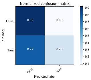
# Plot normalized confusion matrix
plt.figure()
plot_confusion_matrix(cnf_matrix, classes=[False,True], normalize=True,
title='Normalized confusion matrix')
plt.show()
Predicting
In [20]:
y_kasios = clf.predict(X_kasios)
for i in range(len(y_kasios)):
    print("Kasios song n°%s : %s" % (i+1, y_kasios[i]))
The SVM classifier finds that the Kasios songs n°2, 9 and 10 are from Blue Pipit.
In [21]:
from sklearn.ensemble import RandomForestClassifier
In [22]:
clf = RandomForestClassifier(n_estimators=100, max_depth=7)
In [23]:
clf.fit(X_bin_train, y_bin_train)
Out[23]:
Predicting
In [24]:
y_pred_train = clf.predict(X_bin_train)
y_pred_test = clf.predict(X_bin_test)
In [25]:
print(accuracy_score(y_bin_train, y_pred_train))
print("Accuracy: %s" % accuracy_score(y_bin_test,y_pred_test))
In [26]:
# Compute confusion matrix
cnf_matrix = confusion_matrix(y_bin_test, y_pred_test)
np.set_printoptions(precision=2)

# Plot non-normalized confusion matrix
plt.figure()
plot_confusion_matrix(cnf_matrix, classes=[False,True],
                      title='Confusion matrix, without normalization')

# Plot normalized confusion matrix
plt.figure()
plot_confusion_matrix(cnf_matrix, classes=[False,True], normalize=True,
                      title='Normalized confusion matrix')

plt.show()
In [27]:
y_kasios = clf.predict(X_kasios)
In [28]:
print("Classification with Random Forest \n")
for i in range(len(y_kasios)):
    print("Kasios song n°%s : %s"% (i+1, y_kasios[i]))
There is no result from the Random Forest.
Conclusion: Using the binary classification, we can conclude that the Kasios n°9 song has a bigger probability to be a Rose-Crested Blue Pipit one than others. Let's verify if we can get a better result from the Multi Classification.
Conclusion: Using the binary classification, we can conclude that the Kasios n°9 song has a bigger probability to be a Rose-Crested Blue Pipit one than others. Let's verify if we can get a better result from the Multi Classification.
In [48]:
# subsetting just the odd ones
neighbors = list(range(1,50,2))
# empty list that will hold cv scores
cv_scores = []

# perform 10-fold cross validation
for k in neighbors:
    knn = KNeighborsClassifier(n_neighbors=k)
    scores = cross_val_score(knn, X_train, y_train, cv=10, scoring='accuracy')
    cv_scores.append(scores.mean())
# changing to misclassification error
MSE = [1 - x for x in cv_scores]

# determining best k
optimal_k = neighbors[MSE.index(min(MSE))]
print("The optimal number of neighbors is %d" % optimal_k)

# plot misclassification error vs k
plt.plot(neighbors, MSE)
plt.xlabel('Number of Neighbors K')
plt.ylabel('Misclassification Error')
plt.show()
In [30]:
clf = KNeighborsClassifier(n_neighbors=optimal_k)
clf.fit(X_train, y_train)

# Accuracy of the model
accuracy = clf.score(X_test, y_test)
print("Accuracy of the model: %s" % accuracy)
In [31]:
# Compute confusion matrix
y_predict = clf.predict(X_test)
cnf_matrix = confusion_matrix(y_test, y_predict)
np.set_printoptions(precision=2)
# Plot non-normalized confusion matrix
plt.figure(figsize=(20,20))
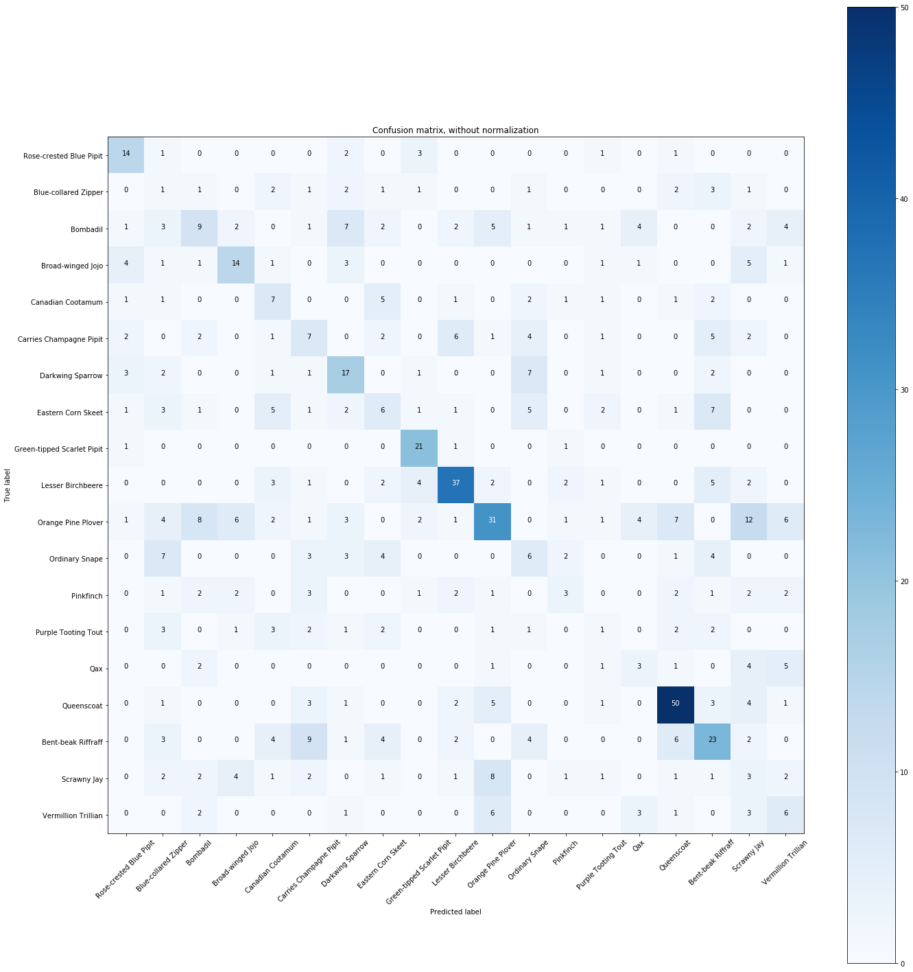
plot_confusion_matrix(cnf_matrix, classes=Y.unique(),
title='Confusion matrix, without normalization')
# Plot normalized confusion matrix
plt.figure(figsize=(20,20))
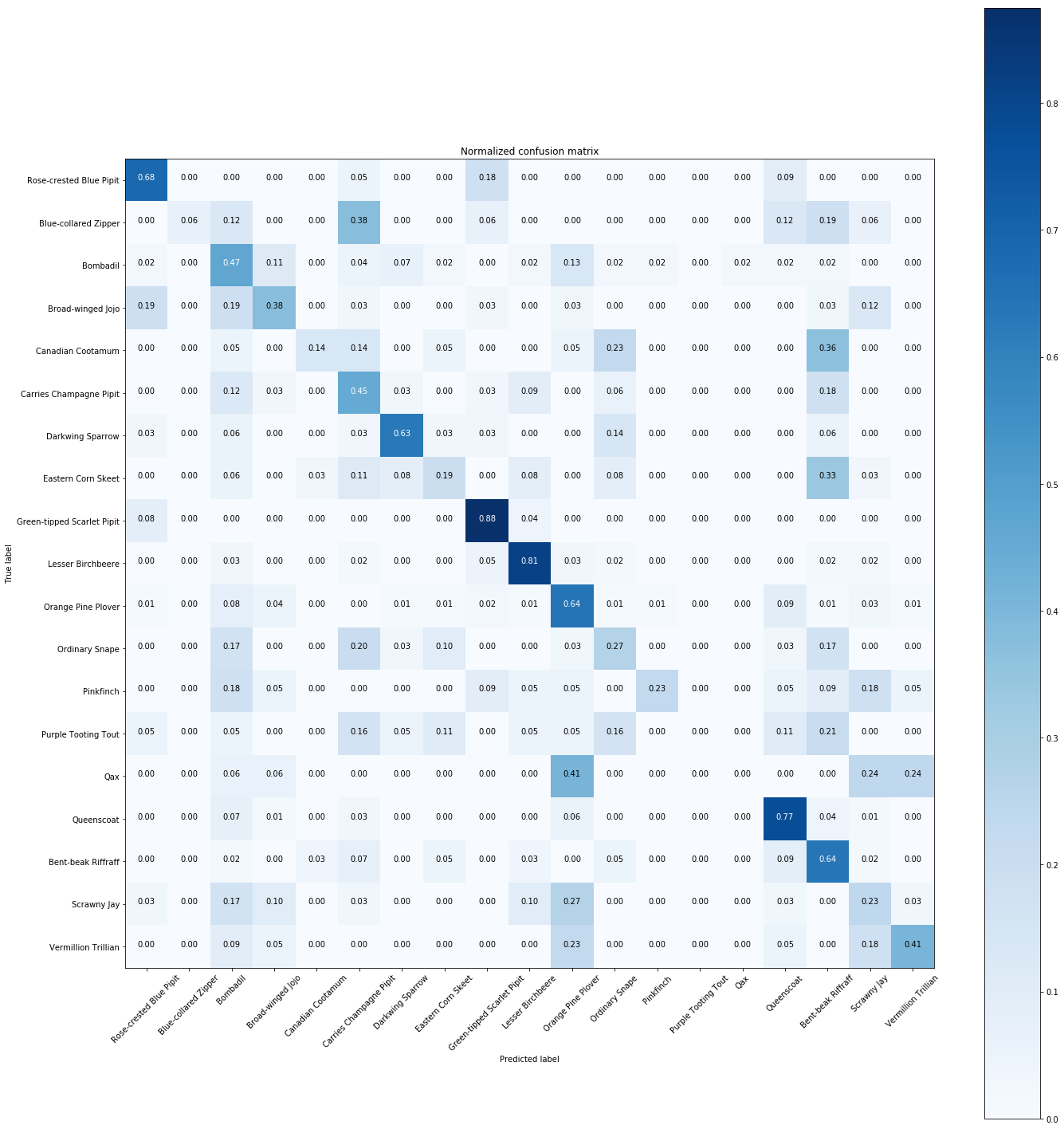
plot_confusion_matrix(cnf_matrix, classes=Y.unique(), normalize=True,
title='Normalized confusion matrix')
plt.show()
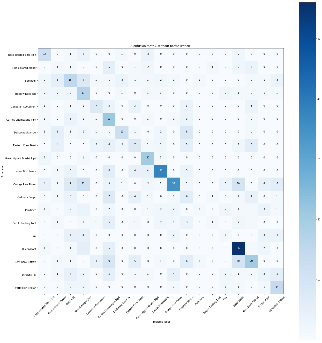
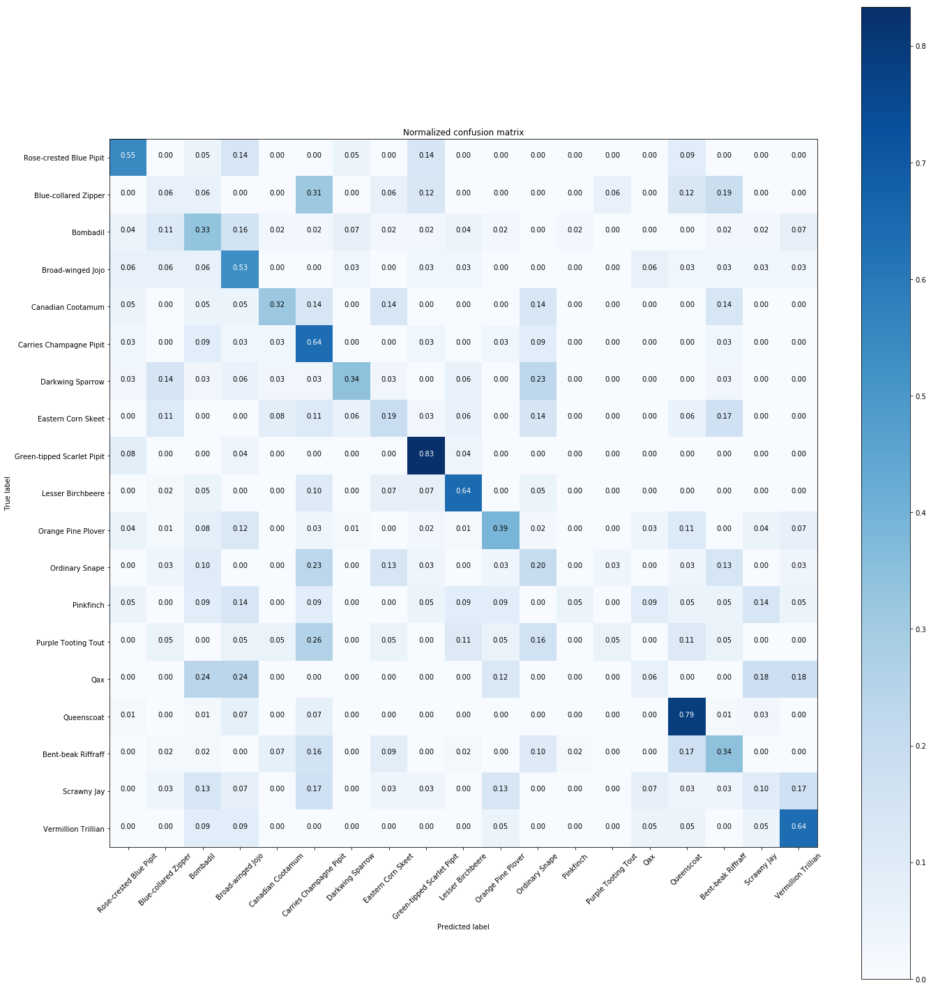
The normalized confusion matrix gives the similarities between species.
Predicting
In [32]:
y_kasios = clf.predict(X_kasios)
for i in range(len(y_kasios)):
    print("Kasios song n°%s : %s" % (i+1, y_kasios[i]))
The kNN classifier finds that the Kasios songs n°2, 9 and 13 are from Blue Pipit.
In [33]:
x_list = np.linspace(2**-5, 2**5, 30)
accuracy_C = []
for x in x_list:
    model = svm.SVC(kernel='linear', C=x)
    model.fit(X_train, y_train)
    accuracy_C.append(model.score(X_test, y_test))
x = 0

# select the C with max accuracy
max_index = accuracy_C.index(max(accuracy_C))
C_chosed = x_list[max_index]
In [34]:
# we do the same thing for gamma

accuracy_gamma = []
for x in x_list:
    model = svm.SVC(kernel='linear', C=C_chosed, gamma=x)
    model.fit(X_train, y_train)
    accuracy_gamma.append(model.score(X_test, y_test))

# to find the C with the max accuracy
max_index = accuracy_gamma.index(max(accuracy_gamma))
gamma_chosed = x_list[max_index]  # the C that we will choose
In [35]:
# We can now define our SVM model
clf = svm.SVC(kernel='linear', C=C_chosed, gamma=gamma_chosed)
clf.fit(X_train, y_train)
Out[35]:
In [36]:
# Accuracy of the model
accuracy = clf.score(X_test, y_test)
print("Accuracy of the model: %s" % accuracy)
In [37]:
# Compute confusion matrix
y_predict = clf.predict(X_test)
cnf_matrix = confusion_matrix(y_test, y_predict)
np.set_printoptions(precision=2)
# Plot non-normalized confusion matrix
plt.figure(figsize=(20,20))
plot_confusion_matrix(cnf_matrix, classes=Y.unique(),
title='Confusion matrix, without normalization')
# Plot normalized confusion matrix
plt.figure(figsize=(20,20))
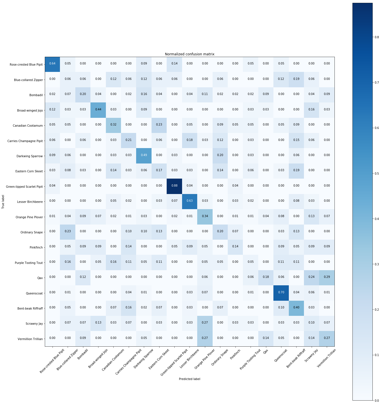
plot_confusion_matrix(cnf_matrix, classes=Y.unique(), normalize=True,
title='Normalized confusion matrix')
plt.show()
Predicting
In [38]:
y_kasios = model.predict(X_kasios)
for i in range(len(y_kasios)):
    print("Kasios song n°%s : %s" % (i+1, y_kasios[i]))
The SVM classifier finds that the Kasios songs n°2 and 13 are from Blue Pipit.
In [39]:
clf = RandomForestClassifier(n_estimators=100, max_depth=7)
clf.fit(X_train, y_train)
Out[39]:
Predicting
In [40]:
# Compute confusion matrix
y_pred_test = clf.predict(X_test)
cnf_matrix = confusion_matrix(y_test, y_pred_test)
np.set_printoptions(precision=2)
# Plot non-normalized confusion matrix
plt.figure(figsize=(20,20))
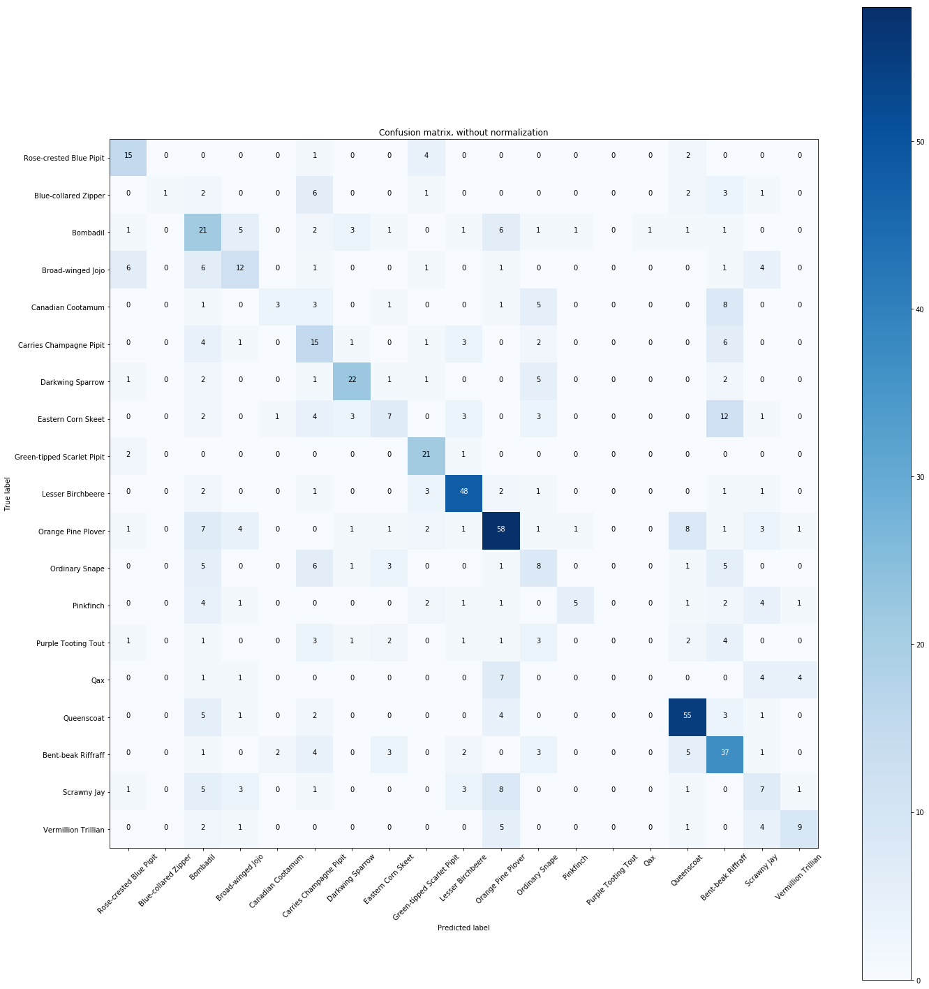
plot_confusion_matrix(cnf_matrix, classes=Y.unique(),
title='Confusion matrix, without normalization')
# Plot normalized confusion matrix
plt.figure(figsize=(20,20))
plot_confusion_matrix(cnf_matrix, classes=Y.unique(), normalize=True,
title='Normalized confusion matrix')
plt.show()
In [41]:
print(accuracy_score(y_train, y_pred_train))
print("Accuracy: %s" % accuracy_score(y_test,y_pred_test))
In [42]:
y_kasios = clf.predict(X_kasios)
In [43]:
print("Classification with Random Forest \n")
for i in range(len(y_kasios)):
    print("Kasios song n°%s : %s"% (i+1, y_kasios[i]))
The Random Forest method finds that the Kasios songs n°2, 9 and 13 are from Blue Pipit.
Conclusion:The multi classification gives a precise result than the binary one. It confirms that the Kasios song n°9 should be a Rose-Crested Blue Pipit song. Furthermore, we can add the n°2 and 13.
III - UMAP (visualization)
In [7]:
import umap

embedding = umap.UMAP(n_neighbors=17).fit_transform(pd.concat([X, X_kasios]))
In [8]:
from bokeh.plotting import figure, show, output_notebook
from bokeh.models import HoverTool, ColumnDataSource, CategoricalColorMapper
from bokeh.palettes import Category20
from bokeh.models import Legend

output_notebook()
In [9]:
df_umap = pd.DataFrame(embedding, columns=('x', 'y'))
df_umap['specie'] = [specie for specie in Y] + ['Kasios Test Bird' for i in range(15)]
df_umap['kasios_index'] = [None for i in Y] + [i for i in range(1, 16)]


plot_figure = figure(
    title='UMAP projection of the birds songs',
    plot_width=800,
    plot_height=600,
    tools=('pan, wheel_zoom, reset'),
    toolbar_location='above'
)

color_mapping = CategoricalColorMapper(factors=df_umap['specie'].unique(),
                                       palette=Category20[20])

plot_figure.add_tools(HoverTool(tooltips="""
<div>
    <div>
        <span style='font-size: 13px; color: #224499'>Specie:</span>
        <span style='font-size: 13px'>@specie</span>
    </div>
</div>
"""))

legend_items = []

for specie in df_umap['specie'].unique():
    datasource = ColumnDataSource(df_umap.loc[df_umap['specie'] == specie])
    if specie == 'Kasios Test Bird':
        c = plot_figure.circle('x', 'y', source=datasource, color='black',
                               line_alpha=0.7, fill_alpha=0.7, size=20)

        plot_figure.text('x', 'y', text='kasios_index', x_offset=-5, y_offset=8,
                         source=datasource, text_font_size='10pt', text_color='white')
    else:
        c = plot_figure.circle('x', 'y', source=datasource,
                               color=dict(field='specie', transform=color_mapping),
                               line_alpha=0.6, fill_alpha=0.6, size=5)

    legend_items.append((specie, [c]))


legend = Legend(items=legend_items, location=(30, 50))
legend.click_policy = 'hide'
plot_figure.add_layout(legend, 'right')

show(plot_figure)
In [10]:
plot_figure = figure(
    title='UMAP projection of the birds songs',
    plot_width=800,
    plot_height=600,
    tools=('pan, wheel_zoom, reset'),
    toolbar_location='above'
)

color_mapping = CategoricalColorMapper(factors=df_umap['specie'].unique(),
                                       palette=Category20[20])

plot_figure.add_tools(HoverTool(tooltips="""
<div>
    <div>
        <span style='font-size: 13px; color: #224499'>Specie:</span>
        <span style='font-size: 13px'>@specie</span>
    </div>
</div>
"""))

legend_items = []

for specie in df_umap['specie'].unique():

    datasource = ColumnDataSource(df_umap.loc[df_umap['specie'] == specie])
    if specie == 'Kasios Test Bird':
        c = plot_figure.circle('x', 'y', source=datasource, color='black',
                               line_alpha=0.7, fill_alpha=0.7, size=20)

        plot_figure.text('x', 'y', text='kasios_index', x_offset=-5, y_offset=8,
                         source=datasource, text_font_size='10pt', text_color='white')
    else:
        c = plot_figure.circle('x', 'y', source=datasource,
                               color=dict(field='specie', transform=color_mapping),
                               muted_color=dict(field='specie', transform=color_mapping),
                               line_alpha=0.6, fill_alpha=0.6, size=5, muted_alpha=0.1)

    legend_items.append((specie, [c]))
    if specie != 'Rose-crested Blue Pipit':
        c.muted = True

legend = Legend(items=legend_items, location=(30, 50))
legend.click_policy = 'hide'
plot_figure.add_layout(legend, 'right')

show(plot_figure)
By using the UMAP method, we can find that some Kasios sounds are in the same area as Rose-crested Blue Pipit (n°2, 9, 11, 13 and 14).
Conclusion:
Through ML methods and the UMAP visualization , we can conclude that the Kasios sounds n°2, 9 and 13 are potentially from Rose-crested Blue Pipit.